Cybernetic Simulation Applet - Instructions
Abstract: This page includes
user's instructions for an applet program made in HUT Control Laboratory.
The aim of the program is to simulate and illustrate a cybernetic ecosystem
that is based on local adaptation. The program implements the "go for
the resources"-behavior. The emergent behavior arising from this strategy
will coincide with sparse- / principal component analysis (with suitable configuration).
More information of the theory is found from the neocybernetics
page.
The program can be easily used without advanced knowledge in
neocybernetics. Below you will find basic instructions to use the program.
For more ambiguous usage, advanced settings can be configured; these are explained
at the end of this page.
Contents:
1.1 Resources
The ecosystem considered consists of plants and herbivores which live in
a closed environment. The environment is considered as a rectangular area
(cf. a half hectare forest) which has a variety of basic resources
(or just resources) which are spatially distributed along the area.
Environment, "The half hectare forest".
The environment has been spatially discretisized so that the resources are
constant in one grid rectangle. The amount of different types of resources
is predetermined (default 8). These could be eg. amount
of sunlight, humidity, fertilizers and so on.
As the environment is spatially discretisized, the whole environment can
now be defined as a 3 dimensional matrix in which the resources are one dimension.
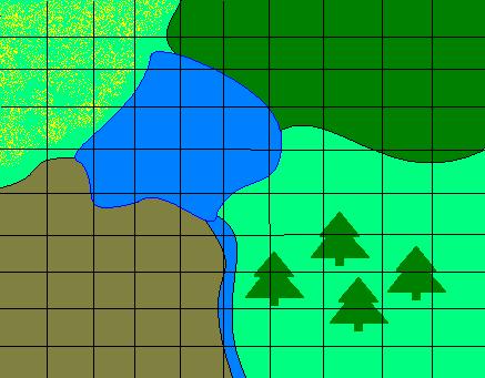
In the program this is visualized with a rectangular map in which the weighting
of different colors illustrates the resources (as shown below).
Environment in the actual program
1.2 Variation in time
The resources are varying in time so that the variation of different resources
is independent, where as there can exist connections between them (cf. high
sunlight results in low humidity). The amount of one resource is varying equally
along the map. Compare to the amount of sunlight; it
varies from place to place, and from year to year but the temporal variation
affects equally along the whole forest.
The resources have nominal values. That is, their average values in time.
These nominal values vary spatially. Compare e.g. that
the humidity close to a river is in average higher. In the program these nominal
values are randomly generated so that they form clusters. In one cluster the
relative distribution of nominal resources are almost equal.
1.3 Profile
The plants (and herbivores) are characterized by their profile. The
profile is a vector of n elements (n resources) that
tell how much the plant benefits of each resource. Compare
to a specific plant that requires little sunlight and much humidity, the profile
would have a small weight on sunlight and a large on humidity (e.g. for [sunlight
humidity] profile [0.1 2.0]).
1.4 Local adaptation
The ecosystem simulation consists of two phases; the local adaptation and
the profile adaptation or the evolution.
The local adaptation timescale is considered relatively fast. In this adaptation
the population sizes and leftover resources are determined independently for
each point. Notice that the profile is considered constant. Compare
to a scenario where e.g. two known plants are competing for the same resources,
the plants will reproduce for as long as the resources last, and the plant
with characteristics better fit for the resources will reproduce more. Iteration
is continued until equilibrium is found. The plant characteristics will not
change in local adaptation.
Local adaptation algorithm
1.5 Profile adaptation
(evolution)
The profile adaptation, that is, the evolution is the adaptation of the plant
core characteristics. The local adaptation is considered to have reached eqilibrium
before the profiles are adapted. Practically, most plants
and herbivores reach local adaptation equilibrium in 1 year, thus the
profile adaptation would happen once a year. The time for the profile to reach
equilibrium is hundreds, thousands of years.
Profile adaptation algorithm
The visual outlook of the plants is a function of the
profile, even though the physical characteristics do not reflect the resource
usage.
2. Instructions
2.1 Running the program
The program runs on java runtime environment 1.4 or newer, with Internet
Explorer or Mozilla browsers. If you encounter problems with the program please
install the newest java runtime environment from http://java.sun.com/javase/downloads/index.jsp
(Java Runtime Environment (JRE) 6 ).
To start the program, click on the link start
simulation. The program will start on a new window. A button "Start
Simulation" is displayed in the middle of the window, press this button
to start the simulation.

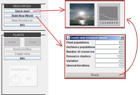
2.2 Initializing resources
First, try “Quick start” button. It will provide a new resource
profile with all settings chosen by computer. If you want to change these
setting, try “Build New World” button.
The environment now created consists of n (default 8) different resources
that are spatially distributed in an area (20 x 20).
There are two different views available for viewing the resources. The default
view is the profile view (below on right). In this view the resources
are shown as collected average over the overall map (20 x 20). The map
view (below on left) shows different resources with different colors spatially
placed on the map. The view can be changed by pressing Toggle view button
while the plants are evolving.

The resources are varying around their nominal values with a chosen variance
(default = 1). The different types of resources are varying independently,
but there is some correlation between them.
The basic resources could be seen to represent sunlight, humidity, fertilizers
and so on.
2.3 Plant evolution
When the resources have been initialized a button START will appear green
on the plants section. Press this START button to start plant evolution.
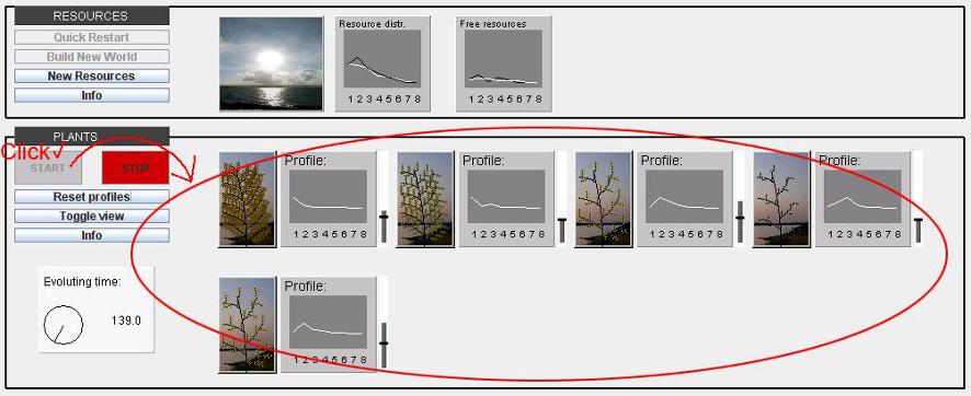
When the START button has been pressed, the evolution will go on until STOP
is pressed. The evolution time (iterations) is shown on the left side of the
window. Each iteration counts for a "year" and only the final balance
is shown.
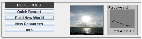
At the beginning of every iteration new current resources are generated
on basis of initialized nominal resources and predetermined variance. The
current resources are shown on the resource section along with the
free resources. The free resources represent the resources that
remain after feedback.
While the evolution is going on you can at any time reset the plant
profiles, initialize new resources or toggle view. Resetting
of profiles will also reset the evolution time.
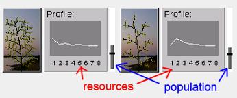
The bar right to the plant profile (or map) represents the current size of
the population. The average size is also shown.
To stop the evolution press STOP. The evolution will stop and you can either
continue the plant evolution, or start the herbivore evolution.
2.4 Herbivore evolution
To start the herbivore evolution, press the green START button in the herbivore
section.
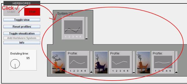
As with the plants, the herbivore evolution will go on until the red STOP
button is pressed. While the evolution is going on you can reset profiles,
toggle view, toggle visualization or initialize new resources.
Resetting the profiles will also reset the evolution timer.
The bar next to the profile represents the size of the herbivore population.
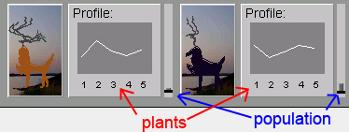
Notice that the herbivores are now using the plants as their resources. The
plants are though not directly varied with time, but through the basic resources.
While evolution is going on, you can also click on any of the herbivore profiles
(or maps) and a new window with additional information will appear. In this
window, you can choose to make the herbivore profile constant by pressing
Set constant profile button. You can adjust the profile by moving the
yellow markers. The profile will be automatically scaled so that its norm
is equal to 1. When you are ready, click ready.
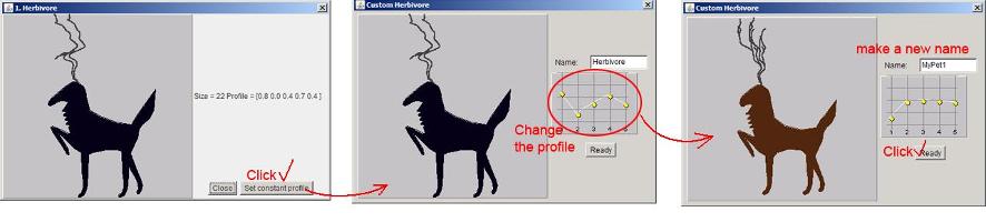
When you have set a profile for a herbivore it will appear among the other
herbivores. The profile of the constant herbivore will be scaled as the evolution
goes on. The scaling will be positive if there are free resources in the direction
of the profile, and negative if there is lack of resources in the direction
of the profile. The appearance of the herbivore does also change as the profile
is scaled.
When you click on the constant herbivore again, a window will appear
that allows you to change the profile. You can also make the herbivore cybernetic
by pressing make cybernetic. If the evolution is going on as you press
make cybernetic it will stop when you press it. When you start the
herbivore evolution again the changed herbivore will act as cybernetic, starting
to evolve from the profile that it had before it became cybernetic.
To stop the herbivore evolution, press the red STOP button.
When the evolution is stopped, you can continue the evolution by pressing
the START button again, continue the plant evolution or add a new herbivore
system by pressing Add Herbivore System. This will add a new, parallel
herbivore system that will evolve simultaneously, independently of the
previous herbivore system. By clicking on the different systems you can get
the system herbivores visible.
2.5 Advanced settings
The program allows you to adjust many simulating parameters. Notice that
changing these parameters might change the emerging behavior of the populations.
To change advanced parameters click "Advanced settings" and "Set
parameters" on the top menu bar. Any on-going simulation will be terminated.
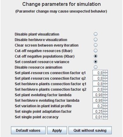
The following parameters affect the simulation:
| Cut-off negative resources (Ubar) |
By selecting this Ubar (current free resources) negative values are set
to zero.
|
| Cut-off negative populations(Xbar) |
By selecting this Xbar (population sizes) negative values
are set to zero. |
| Set constant resource variance |
By selecting this the variance added to different resources
is of equal magnitude, otherwise it is decreasing in power-scale from first
to last resource. |
| Set plant-resources connection factor q1 |
Local adaptation connection factor for plants, see eq.(1) below
|
| Set plant-resources connection factor q2 |
Local adaptation connection factor for plants, see eq.(1)
below |
| Set herbivore-plants connection factor q1 |
Local adaptation connection factor for herbivores, see eq.(1)
below |
| Set herbivore-plants connection factor q2 |
Local adaptation connection factor for herbivores, see eq.(1)
below |
| Set plant evolution factor lambda |
Plant evolution converging factor lambda, see eq.(2) below |
| Set herbivore evolution factor lambda |
Herbivore evolution converging factor lambda, see eq.(2) below |
| Set variation in plant initial profile |
Set the initial variation in plant profiles, also applied
when reset is pressed |
| Set single-point adaptation factor |
Local adaptation converging factor lambda (1&2), see eq.
(1) below |
| Set single point accuracy |
Threshold value for ending local adaptation algorithm, |
Algorithm for local adaptation
| |
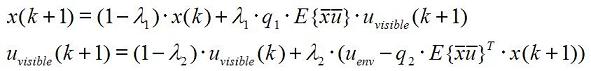 |
(1) |
| |
 population
size , population
size ,  free
(visible) resources, free
(visible) resources,  original
(hidden) resources original
(hidden) resources |
|
| |
 |
|
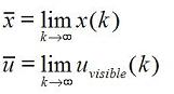
Algorithm for profile
adaptation (evolution):
| |
 |
(2) |
Notice that the above equations include the populations collected in vectors.
The algorithm can also be written in scalar form and the calculations can
be performed independently for each population (in one iterating loop).
2.6 Contact
If you encounter any bugs or have questions about the program implementation,
please contact jan.tiri@tkk.fi.
Ideas on how to develop the program are also welcomed.
Last updated in September 5, 2008 -Jan Tiri